python, 전처리, 통계, 가설검정, 기계학습, 회귀, 분류, 군집, 모델 학습, 모델 평가
상관 분석(Correlation Analysis)은 두 연속형 변수 간의 관계 방향과 강도를 수치로 표현하는 통계적 방법이다. 상관계수는 두 변수가 함께 변하는 패턴을 -1에서 +1 사이의 값으로 나타내며, 변수 간 관계를 탐색하고 이해하는 데 필수적인 도구이다. 이 장에서는 Pearson, Spearman, Kendall 상관계수의 개념과 차이, 그리고 실무 적용 방법을 학습한다.
중요: 상관관계는 두 변수 간 연관성만을 나타내며, 인과관계를 의미하지 않는다.
예제: 데이터 로드
import seaborn as snsimport pandas as pdimport numpy as npimport matplotlib.pyplot as pltfrom scipy import stats# 데이터 로드df = sns.load_dataset("penguins")print("데이터 크기:", df.shape)print("\n연속형 변수:")print(df.select_dtypes(include=[np.number]).columns.tolist())
데이터 크기: (344, 7)

연속형 변수:
['bill_length_mm', 'bill_depth_mm', 'flipper_length_mm', 'body_mass_g']
18.1 상관계수의 기본 개념
상관계수는 두 변수 간 선형 또는 단조 관계의 방향과 강도를 나타낸다.
상관계수의 특성
항목
설명
범위
-1 ≤ r ≤ +1
+1
완벽한 양의 상관 (한 변수 증가 시 다른 변수도 완벽히 증가)
0
선형 관계 없음 (독립적이거나 비선형 관계)
-1
완벽한 음의 상관 (한 변수 증가 시 다른 변수는 완벽히 감소)
|r|
절댓값이 클수록 관계가 강함
상관계수 강도 해석 (경험적 기준)
|r| 값
관계 강도
해석
0.0 ~ 0.1
매우 약함
거의 관계 없음
0.1 ~ 0.3
약함
약한 관계
0.3 ~ 0.5
중간
중간 정도 관계
0.5 ~ 0.7
강함
강한 관계
0.7 ~ 1.0
매우 강함
매우 강한 관계
주의사항
주의점
설명
인과관계 아님
“A와 B가 상관있다” ≠ “A가 B를 야기한다”
이상치 민감
극단값이 상관계수를 크게 왜곡할 수 있음
비선형 관계
비선형 관계는 상관계수가 낮게 나올 수 있음
제3의 변수
두 변수의 상관이 다른 변수 때문일 수 있음
Simpson’s Paradox
전체 데이터와 그룹별 데이터의 상관이 반대일 수 있음
18.2 Pearson 상관계수
Pearson 상관계수는 두 변수 간 선형 관계의 강도와 방향을 측정하는 가장 널리 사용되는 방법이다.
from scipy.stats import pearsonr# 결측치 제거df_corr = df[["bill_length_mm", "bill_depth_mm"]].dropna()print("=== 데이터 정보 ===")print(f"샘플 수: {len(df_corr)}")print("\n기술 통계량:")print(df_corr.describe())
=== 데이터 정보 ===
샘플 수: 342

기술 통계량:
       bill_length_mm  bill_depth_mm
count      342.000000     342.000000
mean        43.921930      17.151170
std          5.459584       1.974793
min         32.100000      13.100000
25%         39.225000      15.600000
50%         44.450000      17.300000
75%         48.500000      18.700000
max         59.600000      21.500000
예제: Pearson 상관계수 계산
# Pearson 상관계수r, p_value = pearsonr( df_corr["bill_length_mm"], df_corr["bill_depth_mm"])print("=== Pearson 상관 분석 ===")print(f"상관계수 (r): {r:.4f}")print(f"p-value: {p_value:.4f}")# 해석alpha =0.05print(f"\n유의수준 {alpha} 기준:")if p_value < alpha:print(f"✓ 상관관계가 통계적으로 유의함")if r >0: direction ="양의"else: direction ="음의"ifabs(r) <0.3: strength ="약한"elifabs(r) <0.5: strength ="중간"else: strength ="강한"print(f" → {direction}{strength} 선형 관계")else:print(f"✗ 상관관계가 통계적으로 유의하지 않음")
=== Pearson 상관 분석 ===
상관계수 (r): -0.2351
p-value: 0.0000

유의수준 0.05 기준:
✓ 상관관계가 통계적으로 유의함
  → 음의 약한 선형 관계
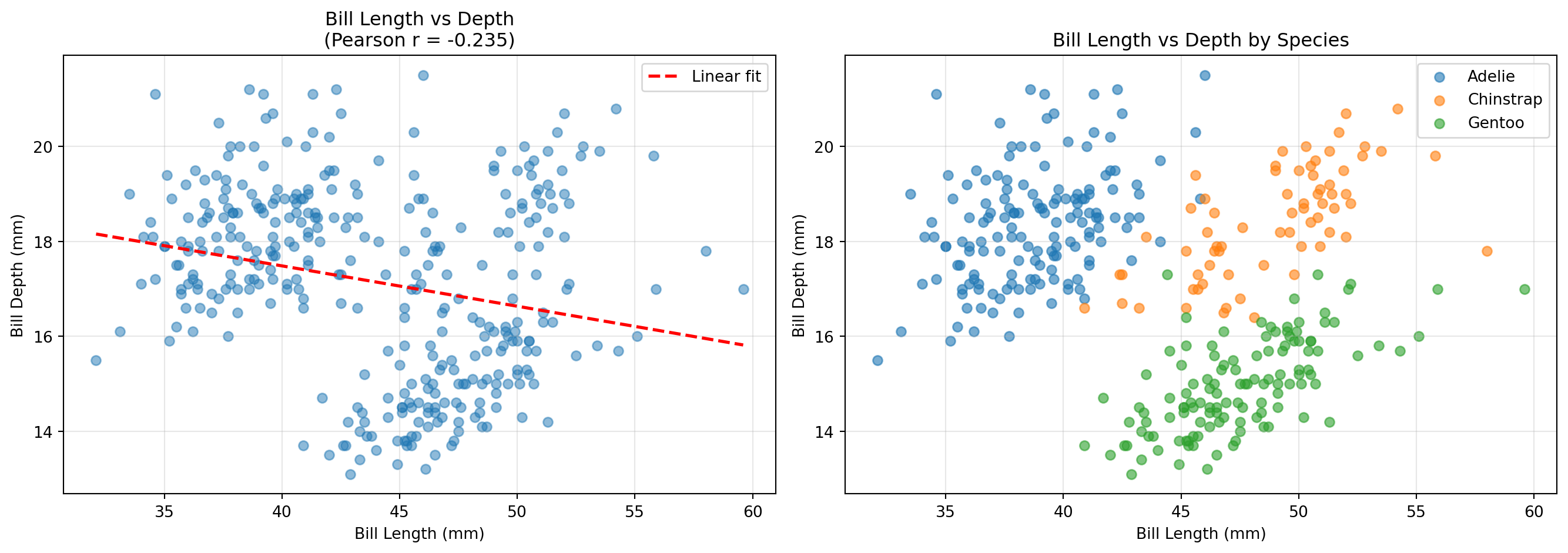
예제: 산점도 시각화
# 산점도와 회귀선fig, axes = plt.subplots(1, 2, figsize=(14, 5))# 전체 데이터 산점도axes[0].scatter(df_corr["bill_length_mm"], df_corr["bill_depth_mm"], alpha=0.5)axes[0].set_title(f"Bill Length vs Depth\n(Pearson r = {r:.3f})")axes[0].set_xlabel("Bill Length (mm)")axes[0].set_ylabel("Bill Depth (mm)")axes[0].grid(True, alpha=0.3)# 회귀선 추가z = np.polyfit(df_corr["bill_length_mm"], df_corr["bill_depth_mm"], 1)p = np.poly1d(z)axes[0].plot(df_corr["bill_length_mm"].sort_values(), p(df_corr["bill_length_mm"].sort_values()), "r--", linewidth=2, label='Linear fit')axes[0].legend()# 종별 산점도 (Simpson's Paradox 확인)for species in df["species"].unique(): species_data = df[df["species"] == species][["bill_length_mm", "bill_depth_mm"]].dropna() axes[1].scatter(species_data["bill_length_mm"], species_data["bill_depth_mm"], alpha=0.6, label=species)axes[1].set_title("Bill Length vs Depth by Species")axes[1].set_xlabel("Bill Length (mm)")axes[1].set_ylabel("Bill Depth (mm)")axes[1].legend()axes[1].grid(True, alpha=0.3)plt.tight_layout()plt.show()
Simpson’s Paradox 확인
# 종별 상관계수print("\n=== 종별 Pearson 상관계수 ===")for species in df["species"].unique(): species_data = df[df["species"] == species][["bill_length_mm", "bill_depth_mm"]].dropna() r_species, p_species = pearsonr(species_data["bill_length_mm"], species_data["bill_depth_mm"])print(f"{species:12s}: r = {r_species:6.3f}, p = {p_species:.4f}")print(f"\n전체 데이터: r = {r:6.3f}, p = {p_value:.4f}")print("\n⚠️ 전체 데이터와 그룹별 상관의 방향이 다를 수 있음 (Simpson's Paradox)")
=== 종별 Pearson 상관계수 ===
Adelie      : r =  0.391, p = 0.0000
Chinstrap   : r =  0.654, p = 0.0000
Gentoo      : r =  0.643, p = 0.0000

전체 데이터:  r = -0.235, p = 0.0000

⚠️ 전체 데이터와 그룹별 상관의 방향이 다를 수 있음 (Simpson's Paradox)
18.3 Spearman 순위 상관계수
Spearman 상관계수는 데이터의 순위를 사용하여 단조 관계를 측정하는 비모수적 방법이다.
개념
측정 대상: 단조 관계 (monotonic relationship)
계산 기반: 순위 간 Pearson 상관계수
가정: 순서형 이상의 데이터, 정규성 불필요
언제 사용하는가?
상황
설명
정규성 위배
데이터가 정규분포를 따르지 않음
이상치 많음
극단값이 결과를 왜곡할 수 있음
비선형 단조 관계
직선은 아니지만 한 방향으로 증가/감소
순서형 데이터
순위나 등급 데이터
가설 설정
H₀ (귀무가설): ρₛ = 0 (두 변수 간 순위 상관이 없다)
H₁ (대립가설): ρₛ ≠ 0 (두 변수 간 순위 상관이 있다)
18.3.1 예제: Spearman 상관계수
예제: Spearman 상관 분석
from scipy.stats import spearmanr# Spearman 순위 상관계수rho, p_value_spear = spearmanr( df_corr["bill_length_mm"], df_corr["bill_depth_mm"])print("=== Spearman 순위 상관 분석 ===")print(f"순위 상관계수 (ρ): {rho:.4f}")print(f"p-value: {p_value_spear:.4f}")# Pearson과 비교print("\n=== Pearson vs Spearman 비교 ===")print(f"Pearson r: {r:.4f} (p = {p_value:.4f})")print(f"Spearman ρ: {rho:.4f} (p = {p_value_spear:.4f})")print(f"차이: {abs(r - rho):.4f}")ifabs(r - rho) >0.1:print("\n⚠️ Pearson과 Spearman 차이가 큼 → 비선형 관계 또는 이상치 의심")
=== Spearman 순위 상관 분석 ===
순위 상관계수 (ρ): -0.2217
p-value: 0.0000

=== Pearson vs Spearman 비교 ===
Pearson r:  -0.2351 (p = 0.0000)
Spearman ρ: -0.2217 (p = 0.0000)
차이: 0.0133
Pearson vs Spearman 비교
항목
Pearson
Spearman
기반
실제 값
순위
측정 관계
선형
단조
이상치 영향
크다
작다
정규성 가정
중요
불필요
계산 복잡도
낮음
중간
적용 범위
선형 관계
단조 관계
18.4 Kendall 순위 상관계수
Kendall τ는 순위 쌍의 일치도를 측정하는 또 다른 비모수적 상관계수이다.
개념
측정 대상: 순위 쌍의 일치 정도
계산 기반: concordant pairs vs discordant pairs
가정: 순서형 이상의 데이터
직관적 설명
두 관측치 쌍 (xᵢ, yᵢ)와 (xⱼ, yⱼ)에 대해: - Concordant: x와 y가 같은 방향으로 증가/감소 - Discordant: x와 y가 반대 방향
from scipy.stats import kendalltau# Kendall τ 계산tau, p_value_kendall = kendalltau( df_corr["bill_length_mm"], df_corr["bill_depth_mm"])print("=== Kendall τ 순위 상관 분석 ===")print(f"Kendall τ: {tau:.4f}")print(f"p-value: {p_value_kendall:.4f}")# 세 가지 상관계수 비교print("\n=== 세 가지 상관계수 비교 ===")print(f"Pearson r: {r:.4f} (p = {p_value:.4f})")print(f"Spearman ρ: {rho:.4f} (p = {p_value_spear:.4f})")print(f"Kendall τ: {tau:.4f} (p = {p_value_kendall:.4f})")print("\n특징:")print("- Kendall τ가 가장 보수적 (절댓값 작음)")print("- 세 계수 모두 같은 방향 (부호 일치)")
=== Kendall τ 순위 상관 분석 ===
Kendall τ: -0.1229
p-value: 0.0008

=== 세 가지 상관계수 비교 ===
Pearson r:  -0.2351 (p = 0.0000)
Spearman ρ: -0.2217 (p = 0.0000)
Kendall τ:  -0.1229 (p = 0.0008)

특징:
- Kendall τ가 가장 보수적 (절댓값 작음)
- 세 계수 모두 같은 방향 (부호 일치)
세 가지 상관계수 종합 비교
구분
Pearson
Spearman
Kendall
기반
실제 값
순위
순위 쌍
측정 관계
선형
단조
단조
이상치 영향
큰
중간
작음
정규성 필요
높음
낮음
낮음
값 크기 경향
가장 큼
중간
가장 작음
해석 안정성
낮음
중간
높음
계산 속도
빠름
중간
느림
동순위 처리
보통
보통
우수
18.5 상관 행렬 (Correlation Matrix)
여러 변수 간의 상관관계를 한눈에 파악할 수 있는 행렬이다.
예제: 상관 행렬 계산
# 수치형 변수 선택num_cols = ["bill_length_mm", "bill_depth_mm", "flipper_length_mm", "body_mass_g"]# Pearson 상관 행렬corr_matrix = df[num_cols].corr(method="pearson")print("=== Pearson 상관 행렬 ===")print(corr_matrix.round(3))
# 상관계수와 p-value를 함께 표시def correlation_with_pvalue(df, method='pearson'):"""상관계수와 p-value를 함께 계산""" corr_matrix = df.corr(method=method) n =len(df)# p-value 행렬 생성 p_matrix = pd.DataFrame(np.zeros_like(corr_matrix), columns=corr_matrix.columns, index=corr_matrix.index)for i, col1 inenumerate(corr_matrix.columns):for j, col2 inenumerate(corr_matrix.columns):if i != j:if method =='pearson': _, p = pearsonr(df[col1].dropna(), df[col2].dropna())elif method =='spearman': _, p = spearmanr(df[col1].dropna(), df[col2].dropna()) p_matrix.iloc[i, j] = preturn corr_matrix, p_matrixcorr, pval = correlation_with_pvalue(df[num_cols], method='pearson')print("=== 상관계수 (위) 및 p-value (아래) ===")for i, col1 inenumerate(num_cols):for j, col2 inenumerate(num_cols):if i < j:print(f"{col1:20s} vs {col2:20s}: r = {corr.iloc[i,j]:6.3f}, p = {pval.iloc[i,j]:.4f}")
=== 상관계수 (위) 및 p-value (아래) ===
bill_length_mm       vs bill_depth_mm       : r = -0.235, p = 0.0000
bill_length_mm       vs flipper_length_mm   : r =  0.656, p = 0.0000
bill_length_mm       vs body_mass_g         : r =  0.595, p = 0.0000
bill_depth_mm        vs flipper_length_mm   : r = -0.584, p = 0.0000
bill_depth_mm        vs body_mass_g         : r = -0.472, p = 0.0000
flipper_length_mm    vs body_mass_g         : r =  0.871, p = 0.0000
18.6 상관 분석 실무 가이드
상관 분석 활용 분야
분야
활용
탐색적 데이터 분석 (EDA)
변수 간 관계 파악
피처 선택
다중공선성 확인, 중복 변수 제거
회귀 모델링
독립변수 선택, 다중공선성 진단
이상치 탐지
예상 밖의 낮은/높은 상관 확인
가설 생성
추가 연구 방향 설정
상관 분석 체크리스트
주의사항
상관 ≠ 인과: “A와 B가 상관있다”는 “A가 B를 야기한다”를 의미하지 않음
비선형 관계: 상관계수가 낮아도 강한 비선형 관계 가능
제3의 변수: 두 변수의 상관이 다른 변수 때문일 수 있음 (교란변수)
Simpson’s Paradox: 전체와 부분에서 상관의 방향이 반대일 수 있음
표본 크기: n이 작으면 우연한 상관이 유의하게 나올 수 있음
18.7 요약
이 장에서는 두 변수 간 관계를 측정하는 상관 분석을 학습했다. 주요 내용은 다음과 같다.
상관계수 종합 정리
상황
권장 방법
이유
선형 관계 + 정규성
Pearson
검정력 높음, 해석 명확
단조 관계 + 비정규
Spearman
정규성 불필요, 이상치 강건
소표본 + 동순위 많음
Kendall
안정적, 동순위 처리 우수
이상치 많음
Spearman 또는 Kendall
Pearson보다 강건
순서형 데이터
Spearman 또는 Kendall
순위 기반
상관 분석 의사결정 흐름
데이터 확인
  ↓
산점도 작성
  ├─ 선형 관계?
  │    ├─ Yes → 정규성 확인
  │    │         ├─ Yes → Pearson
  │    │         └─ No → Spearman
  │    └─ No → 단조 관계?
  │              ├─ Yes → Spearman 또는 Kendall
  │              └─ No → 비선형 모델 고려
  └─ 이상치 많음? → Spearman 또는 Kendall
핵심 포인트
Pearson: 선형 관계의 표준, 가장 널리 사용
Spearman: 단조 관계, 이상치에 강건
Kendall: 보수적, 소표본과 동순위에 강함
상관 ≠ 인과: 항상 주의
시각화 필수: 산점도로 관계 형태 확인
상관 분석은 변수 간 관계를 탐색하고 이해하는 기본 도구이다. 적절한 상관계수를 선택하고, 결과를 올바르게 해석하며, 인과관계로 오해하지 않는 것이 중요하다. 다음으로는 상관 분석을 확장한 회귀 분석을 학습할 수 있다.